大家知道Excel怎么设置自动生成简单甘特图吗?下文小编就带来Excel自动生成简单甘特图的操作方法，一起来看看吧!

      Excel自动生成简单甘特图的操作方法

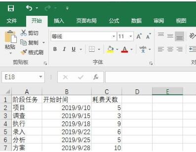
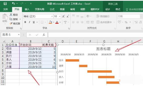
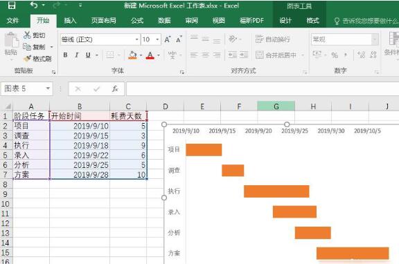
      1、如图所示，首先我们在excel表中输入如下数据。

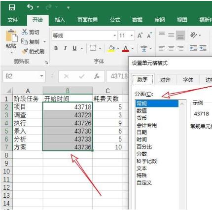
      2、然后我们选中日期这列数据，将其单元格格式设置为常规。

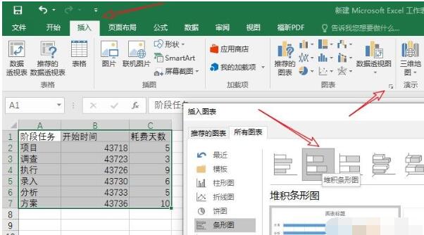
      3、然后我们依此点击excel菜单栏的插入——图表——条形图——堆积条形图。

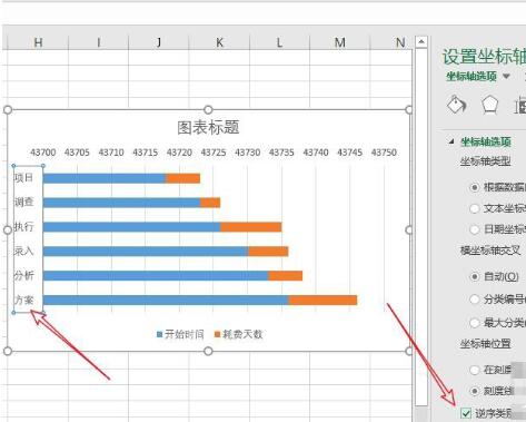
      4、然后我们双击纵坐标——坐标轴选项，勾选逆序类别。

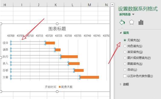
      5、然后我们双击前面的蓝色条形柱，选择填充——无填充。

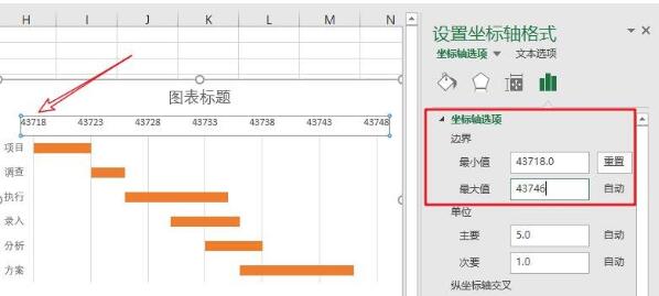
      6、然后我们双击横坐标，点击设置坐标轴选项，最小值设置为步骤一开始时间的最小日期43718，最大值设置为最大日期+耗费天数(43736+10)。

      7、然后我们将开始时间期设置单元格格式为日期，如图所示。

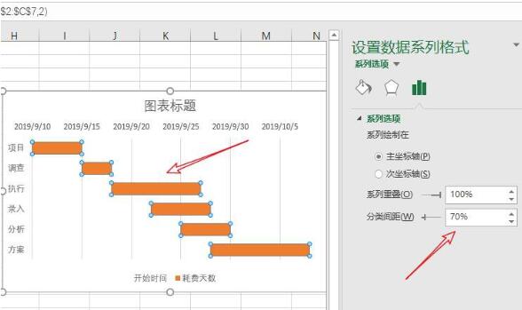
      8、然后双击橙色条形柱，然后选择系列选项——分类间距，设置分类间距可以调整橙色条形柱的粗细，这里我们设置为70%。

      9、最后，我们将一些不必要的如标题，图例删除，就做好一个简单的甘特图了。

      上文就是Excel自动生成简单甘特图的操作方法，赶快试试看吧。